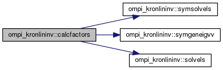
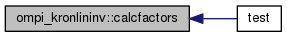
◆ calcfactors()
| subroutine, public ompi_kronlininv::calcfactors | ( | real(dp), dimension(:,:), intent(in) | G1, |
| real(dp), dimension(:,:), intent(in) | G2, | ||
| real(dp), dimension(:,:), intent(in) | G3, | ||
| real(dp), dimension(:,:), intent(in) | Cm1, | ||
| real(dp), dimension(:,:), intent(in) | Cm2, | ||
| real(dp), dimension(:,:), intent(in) | Cm3, | ||
| real(dp), dimension(:,:), intent(in) | Cd1, | ||
| real(dp), dimension(:,:), intent(in) | Cd2, | ||
| real(dp), dimension(:,:), intent(in) | Cd3, | ||
| real(dp), dimension(:,:), intent(out) | U1, | ||
| real(dp), dimension(:,:), intent(out) | U2, | ||
| real(dp), dimension(:,:), intent(out) | U3, | ||
| real(dp), dimension(:), intent(out) | diaginvlambda, | ||
| real(dp), dimension(:,:), intent(out) | iUCm1, | ||
| real(dp), dimension(:,:), intent(out) | iUCm2, | ||
| real(dp), dimension(:,:), intent(out) | iUCm3, | ||
| real(dp), dimension(:,:), intent(out) | iUCmGtiCd1, | ||
| real(dp), dimension(:,:), intent(out) | iUCmGtiCd2, | ||
| real(dp), dimension(:,:), intent(out) | iUCmGtiCd3 | ||
| ) |
Computes the factors necessary to solve the inverse problem.
The factors are the ones to be stored to subsequently calculate posterior mean and covariance. First an eigen decomposition is performed, to get
\[ \mathbf{U}_1 \mathbf{\Lambda}_1 \mathbf{U}_1^{-1} = \mathbf{C}_{\rm{M}}^{\rm{x}} (\mathbf{G}^{\rm{x}})^{\sf{T}} (\mathbf{C}_{\rm{D}}^{\rm{x}})^{-1} \mathbf{G}^{\rm{x}} \]
\[ \mathbf{U}_2 \mathbf{\Lambda}_2 \mathbf{U}_2^{-1} = \mathbf{C}_{\rm{M}}^{\rm{y}} (\mathbf{G}^{\rm{y}})^{\sf{T}} (\mathbf{C}_{\rm{D}}^{\rm{y}})^{-1} \mathbf{G}^{\rm{y}} \]
\[ \mathbf{U}_3 \mathbf{\Lambda}_3 \mathbf{U}_3^{-1} = \mathbf{C}_{\rm{M}}^{\rm{z}} (\mathbf{G}^{\rm{z}})^{\sf{T}} (\mathbf{C}_{\rm{D}}^{\rm{z}})^{-1} \mathbf{G}^{\rm{z}} \]
The principal factors involved in the computation of the posterior covariance and mean are
\[ F_{\sf{A}} = \mathbf{U}_1 \otimes \mathbf{U}_2 \otimes \mathbf{U}_3 \]
\[ F_{\sf{B}} = \big( \mathbf{I} + \mathbf{\Lambda}_1 \! \otimes \! \mathbf{\Lambda}_2 \! \otimes \! \mathbf{\Lambda}_3 \big)^{-1} \]
\[ F_{\sf{C}} = \mathbf{U}_1^{-1} \mathbf{C}_{\rm{M}}^{\rm{x}} \otimes \mathbf{U}_2^{-1} \mathbf{C}_{\rm{M}}^{\rm{y}} \otimes \mathbf{U}_3^{-1} \mathbf{C}_{\rm{M}}^{\rm{z}} \]
\[ F_{\sf{D}} = \left( \mathbf{U}_1^{-1} \mathbf{C}_{\rm{M}}^{\rm{x}} (\mathbf{G}^{\rm{x}})^{\sf{T}} (\mathbf{C}_{\rm{D}}^{\rm{x}})^{-1} \right) \! \otimes \left( \mathbf{U}_2^{-1} \mathbf{C}_{\rm{M}}^{\rm{y}} (\mathbf{G}^{\rm{y}})^{\sf{T}} (\mathbf{C}_{\rm{D}}^{\rm{y}})^{-1} \right) \! \otimes \left( \mathbf{U}_3^{-1} \mathbf{C}_{\rm{M}}^{\rm{z}} (\mathbf{G}^{\rm{z}})^{\sf{T}} (\mathbf{C}_{\rm{D}}^{\rm{z}})^{-1} \right) \]
http://www.netlib.org/lapack/lug/node54.html ?sygst Reduces a real symmetric-definite generalized eigenvalue problem to the standard form.
\(B A z = \lambda z\) B = LLT C = LT A L z = L y
- A is symmetric
- B is symmetric, positive definite
This routines calculates
- Parameters
-
[in] G1,G2,G3 The 3 forward modeling matrices \( \mathbf{G} = \mathbf{G_1} \otimes \mathbf{G_2} \otimes \mathbf{G_3} \) [in] Cm1,Cm2,Cm3,Cd1,Cd2,Cd3 The 6 covariance matrices [out] U1,U2,U3 \( \mathbf{U}_1 \), \( \mathbf{U}_2 \), \( \mathbf{U}_3 \) of \( F_{\sf{A}} \) [out] diaginvlambda \( F_{\sf{B}} \) [out] iUCm1,iUCm2,iUCm3 \(\mathbf{U}_1^{-1} \mathbf{C}_{\rm{M}}^{\rm{x}}\), \(\mathbf{U}_2^{-1} \mathbf{C}_{\rm{M}}^{\rm{y}}\), \(\mathbf{U}_2^{-1} \mathbf{C}_{\rm{M}}^{\rm{z}}\) of \( F_{\sf{C}} \) [out] iUCmGtiCd1,iUCmGtiCd1,iUCmGtiCd1 \( \mathbf{U}_1^{-1} \mathbf{C}_{\rm{M}}^{\rm{x}} (\mathbf{G}^{\rm{x}})^{\sf{T}}(\mathbf{C}_{\rm{D}}^{\rm{x}})^{-1} \), \( \mathbf{U}_2^{-1} \mathbf{C}_{\rm{M}}^{\rm{y}} (\mathbf{G}^{\rm{y}})^{\sf{T}} (\mathbf{C}_{\rm{D}}^{\rm{y}})^{-1}\), \( \mathbf{U}_3^{-1} \mathbf{C}_{\rm{M}}^{\rm{z}} (\mathbf{G}^{\rm{z}})^{\sf{T}} (\mathbf{C}_{\rm{D}}^{\rm{z}})^{-1} \) of \( F_{\sf{D}} \)
- Date
- 10/8/2016 - Initial Version
Definition at line 461 of file ompi_kronlininv.f08.