Traveltimes and rays – using `ttimerays`

Computing travel times and rays through a velocity model is comprised of two main steps:

Discretizing the velocity model on a numerical grid.
Formulating the forward problem of wave front propagation and finding a solution for the discretized model numerically.

PestoSeis offers functions performing both steps and provides additional visualization tools.

Setup of grid parameters and models

In order to compute traveltimes and rays, a 2D grid must be generated to discretize the computational domain. The grid is set up by defining its dimensions in terms of number of cells in the two x and y directions and cell size. Within each cell, the velocity is constant. See pestoseis.ttimerays.setupgrid() for how to create the dictionary holding the grid parameters needed for subsequent computations.

Example:

import pestoseis.ttimerays as tr

# create a 2D grid with 50x30 cells
nx,ny = 50,30
# size of the cells
dh = 5.0
# origin of grid axes
xinit,yinit = 0.0,0.0

# create the dictionary containing the grid parameters
gridpar = tr.setupgrid(nx, ny, dh, xinit, yinit)

Visualization

Some functions for different kinds of plots are provided (click on the function name to get the docstring):

plot the grid: pestoseis.ttimerays.plotgrid()
plot the traveltime array: pestoseis.ttimerays.plotttimemod()
plot the velocity model: pestoseis.ttimerays.plotvelmod()
plot (previously traced) rays: pestoseis.ttimerays.plotrays()

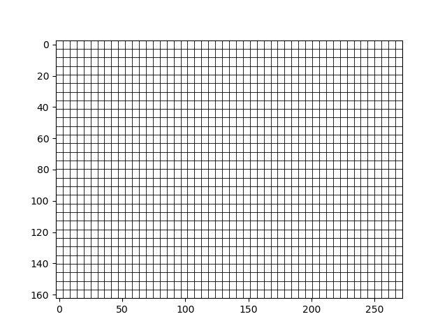
Example of plotting the grid:

import pestoseis.ttimerays as tr
# import the plotting library
import matplotlib.pyplot as pl

# create a 2D grid with 50x30 cells
nx,ny = 50,30
# size of the cells
dh = 5.5
# origin of grid axes
xinit,yinit = 0.0,0.0

# create the dictionary containing the grid parameters
gridpar = tr.setupgrid(nx, ny, dh, xinit, yinit)

# plot the grid
pl.figure()
tr.plotgrid(gridpar)
pl.show()

which produces the following image

Other examples are provided in the following sections.

Computation of traveltimes

One possible way to model wave propagation in a medium is to assume that waves can be approximated by rays of infinite frequency along the path between a source and a receiver. If we consider a specific ray \(i\) along a path \(\Gamma_i\), then we can obtain the traveltime \(t_i\) belonging to that ray by solving the line integral

\[t_i=\int_{\Gamma_i(s(\mathbf{x}))}s(\mathbf{x}(l))dl,\]

where \(\mathbf{x}=[x,y]^{\text{T}}\) in \(\mathbb{R}^2\) and \(s=s(\mathbf{x})\) is the slowness map of the medium and is related to velocity by \(s(\mathbf{x})=\frac{1}{c(\mathbf{x})}\), \(dl\) is an infinitesimal line segment on the path and \(\mathbf{x(}l)\) is the parametrization of the spatial variable in terms of \(l\). To solve this line integral is difficult since it is non-linear in the ray path, which means that the path taken by the ray itself depends on the velocity structure of the medium, which is unknown in realistic experiments. One way to circumvent the explicit need to find ray paths to compute travel times is to decribe the propagation of wavefronts through a medium in 2D with the eikonal equation

\[\left|\nabla t(\mathbf{x})\right|^2=\bigg(\frac{\partial t(\mathbf{x})}{\partial x}\bigg)^2+\bigg(\frac{\partial t(\mathbf{x})}{\partial y}\bigg)^2=s(\mathbf{x})^2,\]

where \(t(\mathbf{x})\) is the traveltime of the wavefront. Note that due to the absolute value, this equation is also non-linear but there exist efficient methods that allow us to solve this partial differential equation equation numerically on a grid. PestoSeis makes use of the Fast Marching Method (FMM), which obtains the traveltime from a source point in a grid to all the other grid points for a given slowness field. In PestoSeis, traveltime calculation given a velocity model and one or more sources and related receivers can be performed using the function pestoseis.ttimerays.traveltime(). By default the function returns both the traveltimes at the receivers and also the entire 2D traveltime array(s) for subsequent ray tracing.

Example:

# import the traveltime-rays sub-module
import pestoseis.ttimerays as tr
import numpy as np
# import the plotting library
import matplotlib.pyplot as pl

# create a 2D grid with 50x30 cells
nx,ny = 50,30
# size of the cells
dh = 5.5
# origin of grid axes
xinit,yinit = 0.0,0.0

# create the dictionary containing the grid parameters
gridpar = tr.setupgrid(nx, ny, dh, xinit, yinit)

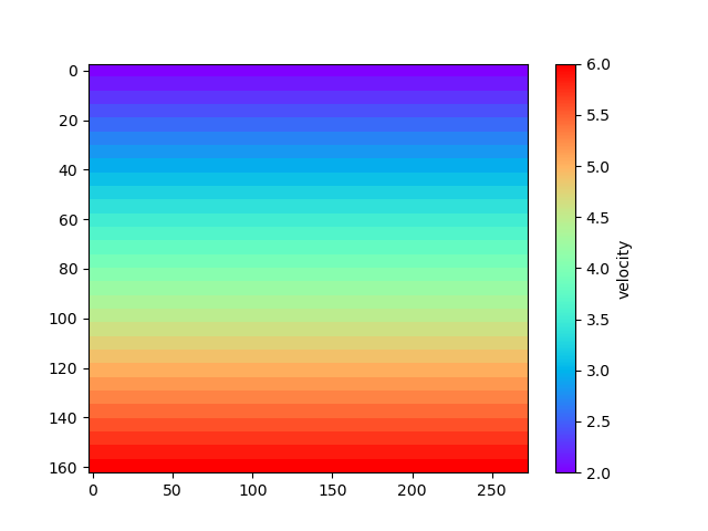
# define a velocity model
velmod = np.zeros((nx,ny))
for i in range(nx):
  velmod[i,:] = np.linspace(2.0,6.0,ny)

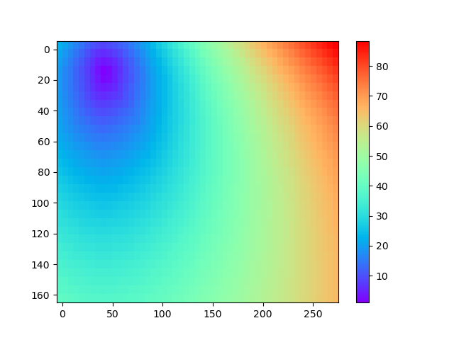
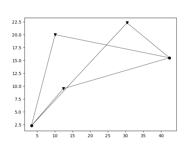
# define the position of sources and receivers, e.g.,
recs = np.array([[30.4, 22.3],
                 [10.1, 20.0],
                 [12.4,  9.5]])
srcs = np.array([[ 3.4,  2.3],
                 [42.4, 15.5]])
## calculate all traveltimes
ttpick,ttime = tr.traveltime(velmod,gridpar,srcs,recs)

ttpick contains an array whose elements are the traveltimes at receivers for each source. In this example we have two sources, hence ttpick has two elements: each of them contains an array with three elements representing the traveltime for each receiver with respect to the source. Similarly, ttime is an array of arrays. In this example we have three sources, so ttime contains three arrays where each of them holds the traveltimes at all grid nodes (for the entire model) for one of the sources.

To plot the velocity model one can use the function pestoseis.ttimerays.plotvelmod():

pl.figure()
tr.plotvelmod(gridpar,velmod)
pl.show()

To plot the resulting traveltimes for a selected source (source #1 in this example), one can use the function pestoseis.ttimerays.plotttimemod():

pl.figure()
tr.plotttimemod(gridpar,ttime[1])
pl.show()

Rays

Trace rays in a 2D heterogeneous model

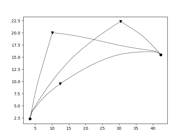
Even though solving the eikonal equation as previously describes results in traveltime information on all grid points without the need to explicitly calculate the ray paths through the medium, there are still stituations where we are interested in obtaining the ray paths between the sources and the receivers. For instance, to set up a tomographic problem, we need to know the length of a ray within each grid cell to set up a sparse tomography matrix. We can make use of the previously computed traveltimes to trace (approximately) the rays using the function pestoseis.ttimerays.traceallrays(). This function traces the rays starting from a receiver position by following the gradient of the traveltimes \(\nabla t(\mathbf{x})\) back through the computed traveltime field to the source. Hence the computed ray path consists of piecewise linear segments (within each grid cell).

Example:

# import the traveltime-rays sub-module
import pestoseis.ttimerays as tr
import numpy as np
# import the plotting library
import matplotlib.pyplot as pl

# create a 2D grid with 50x30 cells
nx,ny = 100,60
# size of the cells
dh = 2.5
# origin of grid axes
xinit,yinit = 0.0,0.0

# create the dictionary containing the grid parameters
gridpar = tr.setupgrid(nx, ny, dh, xinit, yinit)

# define a velocity model
velmod = np.zeros((nx,ny))
for i in range(nx):
  velmod[i,:] = np.linspace(2.0,6.0,ny)

# define the position of sources and receivers, e.g.,
recs = np.array([[30.4, 22.3],
                 [10.1,  20.0],
                 [12.4,  9.5]])
srcs = np.array([[ 3.4,  2.3],
                 [42.4, 15.5]])
## calculate all traveltimes
ttpick,ttime = tr.traveltime(velmod,gridpar,srcs,recs)

## now trace rays (ttime contains a set of 2D traveltime arrays)
rays = tr.traceallrays(gridpar,srcs,recs,ttime)

The computed rays take ray bending in a heterogeneous media into account (in the limit of the grid cell size). The output rays is an array of objects where the number of objects corresponds to the number of receivers. Each object is in turn an array with as many elements as the number of sources. Each of this elements contains all the information relative to a single ray: the coordinates of the points of the ray, the indices of which cells it crosses and the length of the segments in such cells.

The function pestoseis.plotrays() ` is used to visualize the results::

pl.figure()
tr.plotrays(srcs,recs,rays)
pl.show()

Trace straight rays

A very common simplification to the non-linear formulation of the travel time inegral is to invoke the straight-ray approximation by linearizing the integral with respect to the ray path, fixing the geometry of a ray to a straight line between a source and a receiver. This simplifies the integral formulation to

\[t_i=\int_{\Gamma_i}s(\mathbf{x}(l))dl,\]

with \(t_i\) being the traveltime of the ith ray. On the grid, the discrete formulation of this integral is given by the sum

\[t_i=\sum_{j=1}^nl_{ij}s_j,\]

where \(l_{ij}\) is the segment of ray \(i\) in cell \(j\) and \(n\) is the total number of cells. To trace straight rays, use the function pestoseis.ttimerays.traceall_straight_rays().

Example:

# import the traveltime-rays sub-module
import pestoseis.ttimerays as tr
import numpy as np
# import the plotting library
import matplotlib.pyplot as pl

# create a 2D grid with 50x30 cells
nx,ny = 50,30
# size of the cells
dh = 5.5
# origin of grid axes
xinit,yinit = 0.0,0.0

# create the dictionary containing the grid parameters
gridpar = tr.setupgrid(nx, ny, dh, xinit, yinit)

# define a velocity model
velmod = np.zeros((nx,ny))
for i in range(nx):
  velmod[i,:] = np.linspace(2.0,6.0,ny)

# define the position of sources and receivers, e.g.,
recs = np.array([[30.4, 22.3],
                 [10.1,  20.0],
                 [12.4,  9.5]])
srcs = np.array([[ 3.4,  2.3],
                 [42.4, 15.5]])

## now trace straight rays
rays = tr.traceall_straight_rays(gridpar,srcs,recs)

The output rays has the same structure than the output of pestoseis.ttimerays.traceallrays(): see above for a description. The function pestoseis.plotrays() ` is used to visualize the results::

pl.figure()
tr.plotrays(srcs,recs,rays)
pl.show()

Trace rays in a horizontally layered medium

As a third option to trace rays, Pestoseis offers the possibility to compute ray paths, traveltime and the distance covered in a horizonally layered medium. Provided the depths of the layers and their velocity, the function pestoseis.ttimerays.tracerayhorlay() applies Snell’s law \(\text{sin}\theta_1s_1=\text{sin}\theta_2s_2\), with \(\theta_1\) being the angle of incidence in layer 1 with slowness \(s_1\) and \(\theta_2\) being the angle of transmission in layer 2 with slowness \(s_2\), repeatedly for each interface the ray encounters. The geometrical setup is the following:

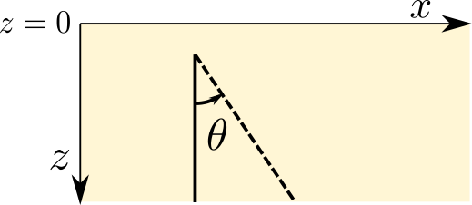
As an input, the angle theta being the take off angle, measured anti-clockwise from the vertical as well as the number of horizontal layers, the depth location of the indicidual interfaces and the velocity within each layer are required.

Example:

import pestoseis.ttimerays as tr
import numpy as np
# number of layers
Nlay = 120
# depth of layers -- includes both top and bottom (Nlay+1)
laydepth = np.linspace(0.0,2000.0,Nlay+1)[1:]
# velocity
vel = np.linspace(2000.0,3000.0,Nlay)
# origin of ray
xystart = np.array([0.0, 0.0])
# take off angle
takeoffangle = 45.0

# trace a single ray
raypath,tt,dist = tr.tracerayhorlay(laydepth, vel, xystart, takeoffangle)

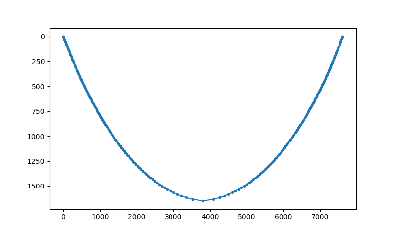
To show the ray path a simple plot can be created::

pl.figure()
pl.plot(raypath[:,0],raypath[:,1],'.-')
pl.gca().invert_yaxis()
pl.show()

Ray tomography

The previously computed traveltimes and rays can be used to set up a tomographic problem. PestoSeis provides the function pestoseis.ttimerays.lininv() to perform a simple linear inversion under Gaussian assumptions (least squares approach). In order to run the inversion the tomography matrix (containing the length of the rays in each cell), the prior mean model and covariances for observed data and model parameters are needed. If we imagine to perform an experiment using a grid of \(n\) cells and a total number of \(m\) source-receiver pairs, resulting in \(m\) rays, then we can leverage the benefit of the linear forward problem by building a linear system of equations

\[\begin{split}\begin{eqnarray} \begin{gathered} t_1=l_{11}s_1+\dots+l_{1j}s_{j}+\dots+l_{1n}s_n \\ \vdots \\ t_i=l_{i1}s_1+\dots+l_{ij}s_{j}+\dots+l_{in}s_n \\ \vdots \\ t_m=l_{m1}s_1+\dots+l_{mj}s_{j}+\dots+l_{mn}s_n. \end{gathered} \end{eqnarray}\end{split}\]

This can be condensed to matrix vector notation by introducing the forward modelling matrix \(\mathbf{G}\) of dimensions \(m\times n\) that collects all line segments \(l_{ij}\) for every source-receiver pair as

\[\mathbf{d}_{\text{obs}}=\mathbf{G}\mathbf{m},\]

where \(\mathbf{d}_{\text{obs}}\) is the vector of observed traveltimes from every source to every receiver and \(\mathbf{m}\) is the model vector containing the slowness map that is supposed to be inferred in the inversion.

After calculating the rays using pestoseis.ttimerays.traceallrays() the tomography matrix \(\mathbf{G}\) can be built subsequently using pestoseis.ttimerays.buildtomomat(). This kind of inversion can be unstable. The model that fits the data best is the one that minimizes the least-squares misfit functional

\[S( \mathbf{m}) = \frac{1}{2} ( \mathbf{G} \mathbf{m} - \mathbf{d}_{\sf{obs}} )^{\sf{T}} \mathbf{C}^{-1}_{\rm{D}} ( \mathbf{G} \mathbf{m} - \mathbf{d}_{\sf{obs}} ) + \frac{1}{2} ( \mathbf{m} - \mathbf{m}_{\sf{prior}} )^{\sf{T}} \mathbf{C}^{-1}_{\rm{M}} ( \mathbf{m} - \mathbf{m}_{\sf{prior}} ).\]

The results are the posterior mean model and covariance matrix (we are under Gaussian assumptions).

The posterior covariance matrix is given by

\[\mathbf{\widetilde{C}}_{\rm{M}} = \left( \mathbf{G}^{\sf{T}} \, \mathbf{C}^{-1}_{\rm{D}} \, \mathbf{G} + \mathbf{C}^{-1}_{\rm{M}} \right)^{-1}\]

and the center of posterior Gaussian (the mean model) is

\[\mathbf{\widetilde{m}} = \mathbf{m}_{\rm{prior}}+ \mathbf{\widetilde{C}}_{\rm{M}} \, \mathbf{G}^{\sf{T}} \, \mathbf{C}^{-1}_{\rm{D}} \left(\mathbf{d}_{\rm{obs}} - \mathbf{G} \mathbf{m}_{\rm{prior}} \right) .\]

The functions provided for performing a tomographic inversion can be used as following. For a complete example see the relevant Jupyter notebook in the Tutorials section.

[...]

# trace rays
rays = tr.traceallrays(gridpar,sources,receivers,bkgttimegrd)
# build the tomography matrix
tomomat,residualsvector = tr.buildtomomat(gridpar, rays, residuals)

# Perform the actual inversion using a "least-squares" approach
postm,postC_m = tr.lininv(tomomat,cov_m,cov_d,mprior,residualsvector)

Traveltimes and rays – using ttimerays

Setup of grid parameters and models

Visualization

Computation of traveltimes

Rays

Trace rays in a 2D heterogeneous model

Trace straight rays

Trace rays in a horizontally layered medium

Ray tomography

Traveltimes and rays – using `ttimerays`