Download This Notebook

Tutorial 02 - Trace rays

import numpy as np
import matplotlib.pyplot as plt
import pestoseis.ttimerays as tr

1. Problem Setup

The objective of this exrcise is to trace a series of rays across a few different input velocity models. First, we start off by importing our data:

i = 3 #1 2 3 4

Changing the value of i will change the input dataset.

filename = f'inputdata/exe2_input_velmod_{i}.npy'
print(filename)

inputdata/exe2_input_velmod_3.npy

inpdat=np.load(filename,allow_pickle=True).item()
gridpar=inpdat['gridpar']
sources=inpdat['srcs']
receivers=inpdat['recs']
velmod=inpdat['velmod']

2. Compute the Traveltimes

Similar to in the previous exercise, we want to compute the traveltimes for the different source-receiver positions.

ttpick,ttime = tr.traveltime(velmod, gridpar, sources, receivers)

Calculating traveltime for source 8 of 8

3. Trace the Rays

Now that we have the traveltimes we can trace the rays to see the ray paths throughout the domain.

rays = tr.traceallrays(gridpar, sources, receivers, ttime)

tracing rays for source 8 of 8

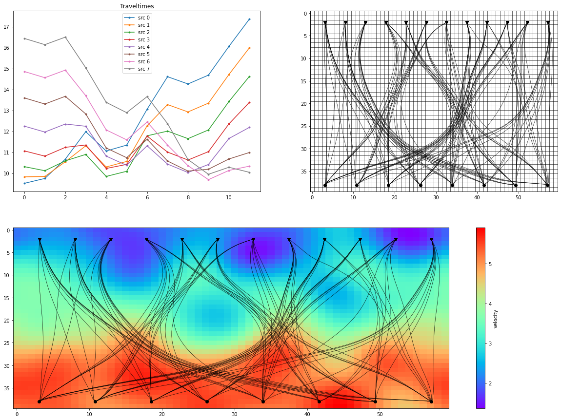
4. Plot the Results

We can not plot the following results:

• The traveltimes for each receiver receiver position

• The ray paths travelled through the domain

import matplotlib.gridspec as gridspec

plt.figure(figsize=(20,15))
gs = gridspec.GridSpec(2, 2)
plt.subplot(gs[0, 0])
plt.title('Traveltimes')
for i in range(ttpick.size):
    plt.plot(ttpick[i][:],'.-',label='src {}'.format(i))
plt.legend()

plt.subplot(gs[0,1])
tr.plotrays(sources,receivers,rays)
tr.plotgrid(gridpar)
#plotttimemod(gridpar,ttime[0])
#extent_ttime = [gridpar['xttmin'],gridpar['xttmax'],
#                gridpar['yttmin'],gridpar['yttmax'] ]
#plt.contour(ttime[0].T,50,extent=extent_ttime,colors='black',linewidth=0.5)

plt.subplot(gs[1,:])
tr.plotvelmod(gridpar,velmod)
tr.plotrays(sources,receivers,rays)

plt.show()

Try to re-run the notebook with different value of i, i.e., with a different input data set.