Tutorial 06 - Elastic Wave Propagation
Elastic Forward Simulation
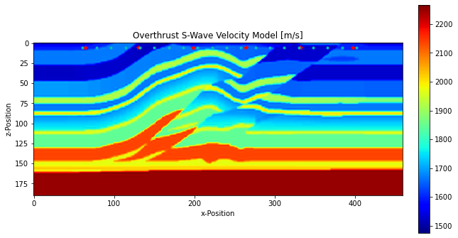
In this notebook we will go through a simple example of setting up an elastic forward simulation in PestoSeis for a 2D portion of the “SEG/EAGE Salt and Overthrust Model” (Aminzadeh et al., 1997).
This notebook will make reference to the acoustic forward simulation example notebook. It is thus suggested to work through the acoustic notebook first before giving the elastic case a try.
Preamble
[1]:
import pestoseis
import numpy as np
import matplotlib.pyplot as plt
import h5py
from scipy.interpolate import RectBivariateSpline
Model Interpolation
Similar to in the acoustic setup, we start by importing the HDF5 (.h5) file containing the velocity model.
[2]:
data_path = "model.h5"
with h5py.File(str(data_path), "r") as f:
    vp = np.array(f["vp"])
    sources = np.array(f["ijsrcs"], dtype=int)
    receivers = np.array(f["ijrecs"], dtype=int)
Since we are considering the same P-wave velocity model in this case as in the purely acoustic case, we will add a conversion using Gardner’s equation given by
where \(\rho\) is density, \(v_p\) is the P-wave velocity, and \(\alpha\) and \(\beta\) are empirically determined quantities. For this example, we will use \(\alpha=0.23\) and \(\beta=0.25\). Care must be taken to first convert \(v_p\) to feet/second (using a conversion factor of 0.3048) and then convert the resulting densities back to metric units in terms of \(\text{kg}/\text{m}^3\).
In order to obtain a test dataset of S-wave velocities, an approximate relationship of
will be considered. Please note that this S-wave relationship is simply being used here for the sake of simplicity and would likely not reflect the actual S-wave velocities one might expect to observe in practice.
As was the case for the purely acoustic setup, the data must be interpolated onto a grid with a finer spatial discretization for use with the 50 kHz source time function.
[3]:
scale = 2

interp_fun = RectBivariateSpline(np.linspace(0, vp.shape[0], vp.shape[0]), np.linspace(0, vp.shape[1], vp.shape[1]), vp)
vp = interp_fun(np.linspace(0, vp.shape[0], vp.shape[0]*scale), np.linspace(0, vp.shape[1], vp.shape[1]*scale))
rho = (0.23 * (vp / 0.3048) ** 0.25)*1000
vs = vp * 3 / 4

sources *= scale
receivers *= scale
Then plotting the results:
[4]:
plt.figure(figsize=[10, 16])
im = plt.imshow(vs.T, origin="upper", cmap="jet")
plt.plot(sources[0, :], sources[1, :], "*r")
plt.plot(receivers[0, :], receivers[1, :], ".c")
plt.xlabel("x-Position")
plt.ylabel("z-Position")
plt.title("Overthrust S-Wave Velocity Model [m/s]")
plt.colorbar(im, fraction=0.046*(10/16), pad=0.04)
plt.show()
Simulation Setup
Next, we can set up the simulation itself. For this example, we will be explicitly defining the following:
Time step
Number of time steps
Source time function characteristics
Free surface boundary conditions at the surface of the domain
PMLs on all other sides
There are two primary differences with this simulation setup compared to the purely acoustic case:
The first derivative of the source must be taken. This is due to the time derivative of the source appearing when obtaining the velocity-stress formulation of the elastic wave equation.
The source is defined in this case as a moment tensor. Here we will set the off-diagonal terms of the moment tensor to be zero and the diagonal elements to be one (for the sake of simplicity). That is,
\[\begin{split}M = \begin{bmatrix} 1.0 & 0.0\\ 0.0 & 1.0 \end{bmatrix}\end{split}\]
[5]:
# Temporal discretizationime
t_sim = 0.3
dt = 0.0005
nt = 2000
t = np.arange(0.0, nt*dt, dt)

# Space
nx = vp.shape[0]
nz = vp.shape[1]
dh = 10 / scale # m

# Source
t0 = 0.03
f0 = 25.0
ijsrc = sources[:, 2]
sourcetf = pestoseis.seismicwaves2d.sourcetimefuncs.ricker_1st_derivative_source( t, t0, f0 )
MTens = dict(xx=1.0, xz=0.0, zz=1.0)

# Receivers
nrec = receivers.shape[1]
recpos = receivers.T * dh

# Lamé coefficients
lamb = rho*(vp**2 - 2.0*vs**2) # P-wave modulus
mu = rho*vs**2 # Shear modulus

print(("Receiver positions:\n{}".format(recpos)))

# Initiallize input parameter dictionary
inpar = {}
inpar["ntimesteps"] = nt
inpar["nx"] = nx
inpar["nz"] = nz
inpar["dt"] = dt
inpar["dh"] = dh
inpar["sourcetype"] = "MomTensor"
inpar["momtensor"] = MTens
inpar["savesnapshot"] = True
inpar["snapevery"] = 50
inpar["freesurface"] = True
inpar["boundcond"] = "PML" #"GaussTap"  ## "PML", "GaussTap","ReflBou"
inpar["seismogrkind"] = "velocity"

# Initiallize dictionary of rock properties
rockprops = {}
rockprops["lambda"] = lamb
rockprops["mu"] = mu
rockprops["rho"] = rho
Receiver positions:
[[ 300.   30.]
 [ 390.   30.]
 [ 480.   30.]
 [ 570.   30.]
 [ 660.   30.]
 [ 750.   30.]
 [ 840.   30.]
 [ 930.   30.]
 [1020.   30.]
 [1110.   30.]
 [1200.   30.]
 [1290.   30.]
 [1380.   30.]
 [1470.   30.]
 [1560.   30.]
 [1650.   30.]
 [1740.   30.]
 [1830.   30.]
 [1920.   30.]
 [2010.   30.]]
Running the Simulation
Now that we have set up the forward simulation, we can run this using solveelastic2D in pestoseis.
[6]:
seism, vxzsave = pestoseis.seismicwaves2d.elasticwaveprop2D.solveelastic2D(inpar, rockprops,ijsrc, sourcetf,f0, recpos)
Starting ELASTIC solver with CPML boundary conditions.
 Source type:  MomTensor
 * Free surface at the top *
 Size of PML layers in grid points: 21 in x and 21 in z
 Time step dt: 0.0005
 Time step 1900 of 2000
Saved elastic simulation and parameters to  elastic_snapshots.h5
Plotting the Results
There are a few different options here for plotting the elastic wavefields:
PS: Plot the P- and S-wavesVxVz: Plot the x- and z-components of the velocity fields seperatelyVmag: Plot the magnitude of the combined velocity componenets
[7]:
h5_data = "elastic_snapshots.h5"
anim = pestoseis.seismicwaves2d.animatewaves.animateelasticwaves(h5_data, showwhatela="VxVz", clipamplitude=0.05)
plt.close(anim._fig)

from IPython.display import HTML
HTML(anim.to_html5_video())
[7]:
References
Aminzadeh, F., Brac, J., Kunz, T., Society of Exploration Geophysicists, & European Association of Geophysicists and Engineers. (1997). 3-D salt and overthrust models. Society of Exploration Geophysicists. https://wiki.seg.org/wiki/SEG/EAGE_Salt_and_Overthrust_Models