Download This Notebook

Tutorial 07 - Processing seismic data I

First let’s import some modules

import numpy as np
import matplotlib.pyplot as plt
import time
import pestoseis.seismicwaves2d as sw
import pestoseis.reflectionseismo as rs

Acoustic waves simulation

Input parameters to run the finite difference code

# time
nt = 4000
dt = 0.0003 #s
t = np.arange(0.0,nt*dt,dt) # s

# space
nx = 438
nz = 240
dh = 3.5 # m

###############################

# source position
lineIdep = 35 #70 # 70
ijsrc = np.array([40,lineIdep])

# receivers
# Create a shotgather, receivers along a horizontal line
nrec = 60
xrec = np.linspace(40*dh,(nx-30)*dh,nrec)
nrec = len(xrec)
recpos = np.zeros((nrec,2))
recpos[:,0] = xrec
recpos[:,1] = (lineIdep)*dh

###############################

# source time function
t0 = 0.07 # s
f0 = 20.0 # Hz

sourcetf = 1e2 * sw.rickersource( t, t0, f0 )
#sourcetf = sw.gaussource( t, t0, f0 )

###############################

## input parameters
inpar={}
inpar["ntimesteps"] = nt
inpar["nx"] = nx
inpar["nz"] = nz
inpar["dt"] = dt
inpar["dh"] = dh
inpar["savesnapshot"] = True
inpar["snapevery"]    = 50
inpar["freesurface"]  = True
inpar["boundcond"]    = "PML"  ## "PML" only choice in this code...

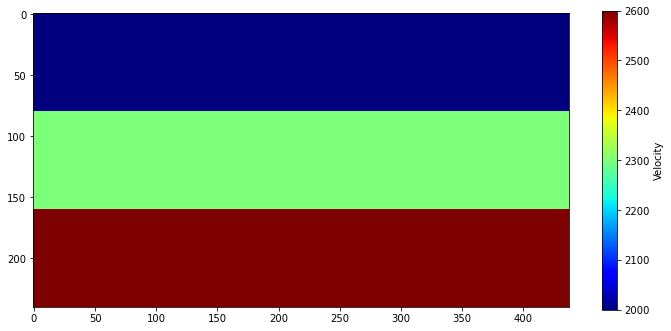
Velocity model

velmod = np.zeros((nx,nz))
velmod[:,:] = 2000.0
velmod[:,80:160] = 2300.0
velmod[:,160:] = 2600.0

plt.figure(figsize=(12,5.5))
plt.imshow(velmod.T,cmap=plt.get_cmap("jet"))
plt.colorbar(label="Velocity")
plt.show()

Run the acoustic simulation

t1 = time.time()
seism,psave = sw.solveacoustic2D( inpar, ijsrc, velmod, sourcetf, f0, recpos )
t2 = time.time()
print(("Solver time: {}".format(t2-t1)))

Starting ACOUSTIC solver with CPML boundary condition.
 Stability criterion, CFL number: 0.3151675939002897
 * Free surface at the top *
 Size of PML layers in grid points: 21 in x and 21 in z
 Time step dt: 0.0003
 Time step 3900 of 4000
Saved acoustic simulation and parameters to  acoustic_snapshots.h5
Solver time: 14.715569019317627

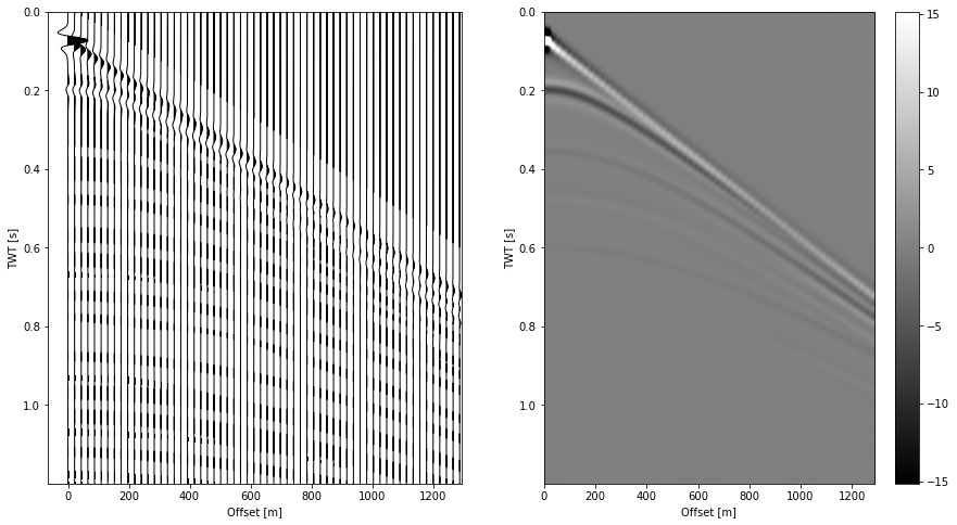
Plot the shotgather

# Compute offset
offset = recpos[:,0]-recpos[0,0]

# Plot shotgather both as image and as wiggles
plt.figure(figsize=(15,8))
plt.subplot(121)
rs.wiggle(seism,dt,offset=offset,scal=3.0)

plt.subplot(122)
vmax = 0.5*np.abs(seism).max()
rs.imgshotgath(seism,dt,offset,amplitudeclip=0.2)

plt.show()

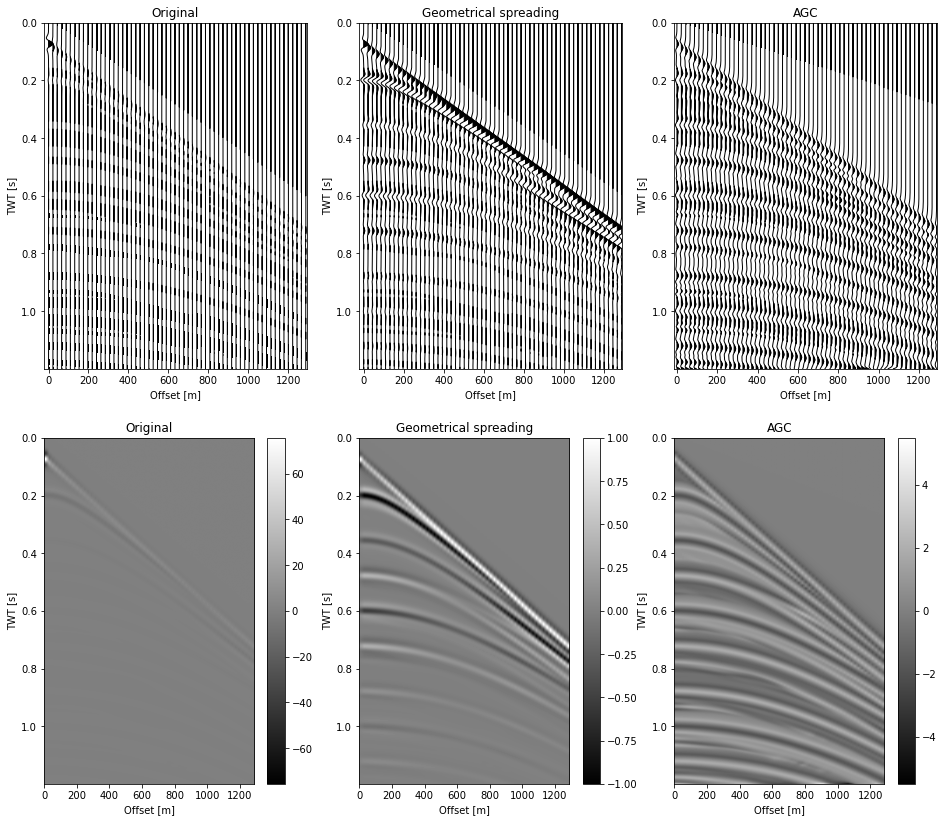
Amplitude enhancement

# TWT array (travel time)
twt = np.arange(0.0,nt*dt,dt)

# Geometrical spreading correction
geomsp = rs.geometrical_spreading(seism,twt)
# Amplitude gain correction (AGC)
agccor = rs.agc(geomsp, w=100)


plt.figure(figsize=(16,14))

plt.subplot(231)
plt.title("Original")
rs.wiggle(seism,dt,offset=offset)

plt.subplot(232)
plt.title("Geometrical spreading")
rs.wiggle(geomsp,dt,offset=offset)

plt.subplot(233)
plt.title("AGC")
rs.wiggle(agccor,dt,offset=offset)

plt.subplot(234)
plt.title("Original")
rs.imgshotgath(seism,dt,offset)

plt.subplot(235)
plt.title("Geometrical spreading")
rs.imgshotgath(geomsp,dt,offset)

plt.subplot(236)
plt.title("AGC")
rs.imgshotgath(agccor,dt,offset)

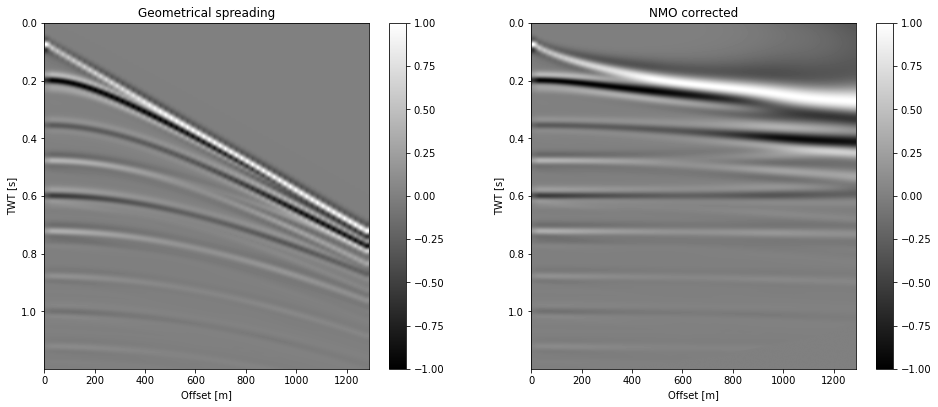
Normal moveout correction

velnmo = np.zeros(seism.shape[1])
velnmo[:] = np.linspace(1850.0,2200.0,seism.shape[1])
snmo = rs.nmocorrection(velnmo,dt,offset,geomsp)


plt.figure(figsize=(16,14))

plt.subplot(221)
plt.title("Geometrical spreading")
rs.imgshotgath(geomsp,dt,offset,amplitudeclip=1)

plt.subplot(222)
plt.title("NMO corrected")
rs.imgshotgath(snmo,dt,offset,amplitudeclip=1)

#rs.wiggle(snmo,dt,offset=offset)

Create a movie

#%matplotlib notebook


anim = sw.animateacousticwaves("acoustic_snapshots.h5",clipamplitude=0.1,showanim=False)
plt.close(anim._fig)

from IPython.display import HTML
HTML(anim.to_html5_video())