Download This Notebook

Tutorial 05 - Acoustic Wave Propagation

Acoustic Forward Simulation

In this notebook we will go through a simple example of setting up a purely acoustic forward simulation in PestoSeis for a 2D portion of the “SEG/EAGE Salt and Overthrust Model” (Aminzadeh et al., 1997).

Preamble

import pestoseis
import numpy as np
import matplotlib.pyplot as plt
import h5py
from scipy.interpolate import RectBivariateSpline

Model Interpolation

First, we will import the HDF5 (.h5) model which contains the following keys:

• vp: P-wave velocity model (in units of [m/s])

• ijsrcs: Indices of the source positions

• ijrecs: Indices of the receiver positions

data_path = "model.h5"
with h5py.File(str(data_path), "r") as f:
    vp = np.array(f["vp"])
    sources = np.array(f["ijsrcs"], dtype=int)
    receivers = np.array(f["ijrecs"], dtype=int)

We can plot the velocity model to verify that the data has been imported correctly.

plt.figure(figsize=[10, 16])
im = plt.imshow(vp.T, origin="upper", cmap="jet")
plt.plot(sources[0, :], sources[1, :], "*r")
plt.plot(receivers[0, :], receivers[1, :], ".c")
plt.xlabel("x-Position")
plt.ylabel("z-Position")
plt.title("Overthrust P-Wave Velocity Model [m/s]")
plt.colorbar(im, fraction=0.046*(10/16), pad=0.04)
plt.show()

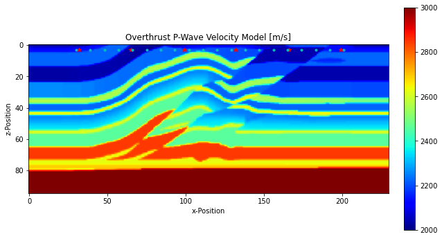
Notice that the P-wave velocity model is currently fairly coarse (ie. there are relatively few samples in the x- and z-directions). This discretisation is currently too coarse for the desired source frequency we want to use for this example (50 Hz), so we need to interpolate this coarser model onto a finer grid. A fairly simple way of accomplishing this is to use the RectBivariateSpline tool from the scipy package.

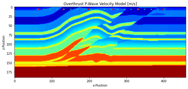
We can set a desired scaling factor (see scale) which will scale the number of samples in each of the x- and z-directions.

scale = 2

interp_fun = RectBivariateSpline(np.linspace(0, vp.shape[0], vp.shape[0]), np.linspace(0, vp.shape[1], vp.shape[1]), vp)
vp = interp_fun(np.linspace(0, vp.shape[0], vp.shape[0]*scale), np.linspace(0, vp.shape[1], vp.shape[1]*scale))

sources *= scale
receivers *= scale

plt.figure(figsize=[10, 16])
plt.imshow(vp.T, origin="upper", cmap="jet")
plt.plot(sources[0, :], sources[1, :], "*r")
plt.plot(receivers[0, :], receivers[1, :], ".c")
plt.xlabel("x-Position")
plt.ylabel("z-Position")
plt.title("Overthrust P-Wave Velocity Model [m/s]")
plt.show()

Simulation Setup

Next, we can set up the simulation itself. For this example, we will be explicitly defining the following:

• Time step

• Number of time steps

• Source time function characteristics (Ricker wavelet)

• Free surface boundary conditions at the surface of the domain

• PMLs on all other sides

# Temporal discretization
nt = 2000
dt = 0.0005
t = np.arange(0.0, nt*dt, dt)

# Spatial discretization
nx = vp.shape[0]
nz = vp.shape[1]
dh = 10 / scale

# Sources
t0 = 0.03
f0 = 25.0
ijsrc = sources[:, 2]

# Source time function
sourcetf = pestoseis.seismicwaves2d.sourcetimefuncs.rickersource( t, t0, f0 )

# Receivers
nrec = receivers.shape[1]
recpos = receivers.T * dh

print(("Receiver positions:\n{}".format(recpos)))

# Initiallize input parameter dictionary
inpar = {}
inpar["ntimesteps"] = nt
inpar["nx"] = nx
inpar["nz"] = nz
inpar["dt"] = dt
inpar["dh"] = dh
inpar["savesnapshot"] = True
inpar["snapevery"] = 50
inpar["freesurface"] = True
inpar["boundcond"] = "PML" #"GaussTap", "PML", "GaussTap","ReflBou"

Receiver positions:
[[ 300.   30.]
 [ 390.   30.]
 [ 480.   30.]
 [ 570.   30.]
 [ 660.   30.]
 [ 750.   30.]
 [ 840.   30.]
 [ 930.   30.]
 [1020.   30.]
 [1110.   30.]
 [1200.   30.]
 [1290.   30.]
 [1380.   30.]
 [1470.   30.]
 [1560.   30.]
 [1650.   30.]
 [1740.   30.]
 [1830.   30.]
 [1920.   30.]
 [2010.   30.]]

Running the Simulation

Now that we have set up the forward simulation, we can run this using solveacoustic2D in pestoseis.

seism, psave = pestoseis.seismicwaves2d.acousticwaveprop2D.solveacoustic2D(inpar, ijsrc, vp, sourcetf, f0, recpos)

Starting ACOUSTIC solver with CPML boundary condition.
 Stability criterion, CFL number: 0.42734622684758544
 * Free surface at the top *
 Size of PML layers in grid points: 21 in x and 21 in z
 Time step dt: 0.0005
 Time step 1900 of 2000
Saved acoustic simulation and parameters to  acoustic_snapshots.h5

Plotting the Results

h5_data = "acoustic_snapshots.h5"
anim = pestoseis.seismicwaves2d.animatewaves.animateacousticwaves(h5_data, clipamplitude=0.1)
plt.close(anim._fig)

from IPython.display import HTML
HTML(anim.to_html5_video())

References

Aminzadeh, F., Brac, J., Kunz, T., Society of Exploration Geophysicists, & European Association of Geophysicists and Engineers. (1997). 3-D salt and overthrust models. Society of Exploration Geophysicists. https://wiki.seg.org/wiki/SEG/EAGE_Salt_and_Overthrust_Models